Contours

Contours are curves joining point along a boundary having same colour or intensity. To accurately use the contour features, use a binary image. Since the findContours function modifies the original image always backup the original image in a separate variable. Also the object to be detected should white on a black background.

Once the image binarization is done, Contour detection can be carried out.
The findContours() function uses 3 arguments: First is the image, second the contour retrieval mode, third is contour approximation method. The outputs are the image,contours and hierarchy. Contours is a list of all the contours in the image. Each contour is an array of the coordinates making the contour.

To draw the contours we use the drawContours function. It takes as argument: the image name, the Python list containing all the contours generated by findContours, the index of the contour to draw and the colour and thickness of the boundary.

The contour approximation method is the third parameter in the findContours function. It can be set to cv2.CHAIN_APPROX_NONE which detects and saves all the boundary points in the contour or cv2.CHAIN_APPROX_SIMPLE which only saves the end points of the contour. The latter removes redundancy and also saves memory.

Canny Edge Detection

Edges are one of the most important features in an image. Edges are basically areas with high intensity contrast. Canny edge detection algorithm developed by John F. Canny in 1986 is a multi-stage optimal edge detector. It is carried out as follows:

Noise Reduction
Since every image is susceptible to noise a Gaussian filter is applied and the image is smoothed.

Intensity Gradient
A Sobel filter is applied to smoothed image in both x and the y axis. This gives the edge gradients and direction of the edge pixels.

Non-maximum Suppression
Every pixel extracted out by the Sobel filter is tested for whether it constitutes an edge or not.
This is done by testing if the pixel is at a local maximum in its neighbourhood in the direction of gradient.
This step basically thins out the edges.

Hysteresis Thresholding
This final tests if all the detected edges are real or dummy. Two threshold values minVal and maxVal are set. Any edge with intensity gradient above maxVal is an edge an those below minVal are discarded. The pixels which lie in between if are discarded if they are not connected to a sure edge.

A simple example to show how Canny edge detection is carried out using python:

import cv2
import numpy as np
from matplotlib import pyplot as plt

img = cv2.imread('circle.png',0)
edges = cv2.Canny(img,100,200)

plt.subplot(121),plt.imshow(img,cmap = 'gray')
plt.title('Original Image'), plt.xticks([]), plt.yticks([])
plt.subplot(122),plt.imshow(edges,cmap = 'gray')
plt.title('Edge Image'), plt.xticks([]), plt.yticks([])

plt.show()


The result:

An application for Canny Edge detection with trackbars to adjust the Hysteresis threshold values:
Canny_Edge_detector.git

Sayonara!!

OpenCV+Python:Part3–Image Gradients

In this post I will explain the application of Gradient or High pass Filters namely Sobel, Scharr and Laplacian

Sobel and Scharr

These perform Gaussian smoothing and differentiation operation and hence provides resistance against noise. The direction of the differentiation can be specified within the function along with the kernel size.

Laplacian

This calculates the laplacian of the image where the derivative at each position is found using the sobel derivatives

The following code snippet describes the use of the above given derivatives and gives an output of np.uint8 type with a kernel size of 5×5 —


import cv2
import numpy as np
from matplotlib import pyplot as plt
img = cv2.imread('image.jpg',0)
laplacian = cv2.Laplacian(img,cv2.CV_64F)
sobelx = cv2.Sobel(img,cv2.CV_64F,1,0,ksize=5)
sobely = cv2.Sobel(img,cv2.CV_64F,0,1,ksize=5)
plt.subplot(2,2,1),plt.imshow(img,cmap = 'gray')
plt.title('Original'), plt.xticks([]), plt.yticks([])
plt.subplot(2,2,2),plt.imshow(laplacian,cmap = 'gray')
plt.title('Laplacian'), plt.xticks([]), plt.yticks([])
plt.subplot(2,2,3),plt.imshow(sobelx,cmap = 'gray')
plt.title('Sobel X'), plt.xticks([]), plt.yticks([])
plt.subplot(2,2,4),plt.imshow(sobely,cmap = 'gray')
plt.title('Sobel Y'), plt.xticks([]), plt.yticks([])
plt.show()


The result–

One important thing to note in the above example is that the data type of the result image is taken as np.uint8 in which all Black to White transitions are considered Positive slopes but all the White to Black transitions are taken as Negative slope and hence are taken as zero in the final result and important edge information is lost. However if you want to keep the edge info intact you can use a higher data type like cv2.CV_16S, cv2.CV_64F etc, take its absolute value and convert it back to cv2.CV_8U.

The following code snippet demonstrates this procedure by applying a horizontal Sobel filter :


import cv2
import numpy as np
from matplotlib import pyplot as plt
img = cv2.imread('image.jpg',0)
# Output dtype = cv2.CV_8U
sobelx8u = cv2.Sobel(img,cv2.CV_8U,1,0,ksize=5)
# Output dtype = cv2.CV_64F. Then take its absolute and convert to cv2.CV_8U
sobelx64f = cv2.Sobel(img,cv2.CV_64F,1,0,ksize=5)
abs_sobel64f = np.absolute(sobelx64f)
sobel_8u = np.uint8(abs_sobel64f)
plt.subplot(1,3,1),plt.imshow(img,cmap = 'gray')
plt.title('Original'), plt.xticks([]), plt.yticks([])
plt.subplot(1,3,2),plt.imshow(sobelx8u,cmap = 'gray')
plt.title('Sobel CV_8U'), plt.xticks([]), plt.yticks([])
plt.subplot(1,3,3),plt.imshow(sobel_8u,cmap = 'gray')
plt.title('Sobel abs(CV_64F)'), plt.xticks([]), plt.yticks([])
plt.show()


The result:

That’s all in this post…Sayonara!!

OpenCV+Python:Part3–Smoothing Images

In this post I will explain the low pass filters available in OpenCV. A low pass filter or an LPF is basically used in reducing the noise and/or blurring the image.

2D Convolution Filtering

In this method a window of 5×5 is formed around every pixel and the average is calculated of the value of the pixels falling within this window.This is done by using the cv2.filter2D() to convolve a kernel with an image
The following code snippet shows how to carry out the filtering:


import cv2
import numpy as np
from matplotlib import pyplot as plt
img = cv2.imread('image.jpg')
kernel = np.ones((5,5),np.float32)/25
dst = cv2.filter2D(img,-1,kernel)
plt.subplot(121),plt.imshow(img),plt.title('Original')
plt.xticks([]), plt.yticks([])
plt.subplot(122),plt.imshow(dst),plt.title('Averaging')
plt.xticks([]), plt.yticks([])
plt.show()


The result–

Image Blurring

Image blurring is achieved by applying a LPF. It basically removes the high frequency content basically noise.

1.)Averaging

This method simply takes a window of 3×3 and replaces the central pixel by the average value of this window using the cv2.blur() or cv2.boxFilter() function.

The following example shows how blurring is carried out:


import cv2
import numpy as np
from matplotlib import pyplot as plt
img = cv2.imread('image.jpg')
blur = cv2.blur(img,(5,5))
plt.subplot(121),plt.imshow(img),plt.title('Original')
plt.xticks([]), plt.yticks([])
plt.subplot(122),plt.imshow(blur),plt.title('Blurred')
plt.xticks([]), plt.yticks([])
plt.show()


The result:

2.)Gaussian Filtering

In this method the height and width of the kernel(window) is passed into the function along with standard deviation along the X and Y directions. The height and width passed must be odd values and the deviations may be passed separately. If only one deviation is passed then both of them are considered equal. If no deviation is given, the function decides them on basis of the window(kernel) size.

Just modifying the above averaging code by replacing the blur statement with
blur = cv2.GaussianBlur(img,(5,5),0) will do the trick.

Result:

3.)Median Filtering

In this case the median of the kernel window is decided and this value is assigned to the central pixel. In case of Gaussian filtering a value that does not exist in the original image may also be assigned, however in case of median filtering the value of the central pixel is always replaced by some pixel value from the image.

Just modifying the above averaging code by replacing the blur statement with
blur = cv2.medianBlur(img,5) will do the trick.

Result:

4.)Bilateral Filtering

In every other case the while blurring the edges along with noise also got blurred in the process. However the function cv2.bilateralFilter() is highly effective in removing noise while preserving the edges.
The bilateral filter uses the very same Gaussian technique except that now it also includes one more component. The Gaussian function defines a kernel and carries out the filtering considering only the kernel space, however this new component that applies to bilateral filtering uses intensity difference to define the kernel space thereby including pixels in the same intensity region. Therefore pixels lying at the edges displaying large intensity variations will not be included in the blurring and hence be preserved.

Just modifying the above averaging code by replacing the blur statement with
blur = cv2.bilateralFilter(img,9,75,75) will do the trick.

Result:

That’s all in this post!! Sayonara.

Otsu’s Binarization

For global thresholding methods we gather the threshold values by trial and error. However suppose the image is Bimodal(Basically a bimodal image has two peaks in its histogram). For this the threshold value is gained by taking the value in between the peaks. This is what is done by Otsu’s Binarization. To use it we simply pass an extra flag cv2.THRESH_OTSU to the cv2.threshold function. Pass the maxVal as 0.


import cv2
import numpy as np
from matplotlib import pyplot as plt

img = cv2.imread('image.jpg',0)

# global thresholding
ret1,th1 = cv2.threshold(img,127,255,cv2.THRESH_BINARY)

# Otsu's thresholding
ret2,th2 = cv2.threshold(img,0,255,cv2.THRESH_BINARY+cv2.THRESH_OTSU)

# Otsu's thresholding after Gaussian filtering
blur = cv2.GaussianBlur(img,(5,5),0)
ret3,th3 = cv2.threshold(blur,0,255,cv2.THRESH_BINARY+cv2.THRESH_OTSU)

# plot all the images and their histograms
images = [img, 0, th1,
img, 0, th2,
blur, 0, th3]
titles = ['Original Noisy Image','Histogram','Global Thresholding (v=127)',
'Original Noisy Image','Histogram',"Otsu's Thresholding",
'Gaussian filtered Image','Histogram',"Otsu's Thresholding"]

for i in xrange(3):
plt.subplot(3,3,i*3+1),plt.imshow(images[i*3],'gray')
plt.title(titles[i*3]), plt.xticks([]), plt.yticks([])
plt.subplot(3,3,i*3+2),plt.hist(images[i*3].ravel(),256)
plt.title(titles[i*3+1]), plt.xticks([]), plt.yticks([])
plt.subplot(3,3,i*3+3),plt.imshow(images[i*3+2],'gray')
plt.title(titles[i*3+2]), plt.xticks([]), plt.yticks([])
plt.show()


The result:

OpenCV+Python:Part3–Image Thresholding

Simple Thresholding

This is as simple as it sounds. You take a threshold pixel value. Anything above(or below) that value is assigned a certain predefined pixel value that you wish. The function cv2.threshold is used .
The function has four parameters. The first is the source image. Second is the threshold value. Third is the maxVal which is the pixel value assigned if the current value is above(or below) the threshold. The fourth parameter is the style in which thresholding can be performed.


import cv2
import numpy as np
from matplotlib import pyplot as plt

img = cv2.imread('image.jpg',0)
ret,thresh1 = cv2.threshold(img,127,255,cv2.THRESH_BINARY)
ret,thresh2 = cv2.threshold(img,127,255,cv2.THRESH_BINARY_INV)
ret,thresh3 = cv2.threshold(img,127,255,cv2.THRESH_TRUNC)
ret,thresh4 = cv2.threshold(img,127,255,cv2.THRESH_TOZERO)
ret,thresh5 = cv2.threshold(img,127,255,cv2.THRESH_TOZERO_INV)

titles = ['Original Image','BINARY','BINARY_INV','TRUNC','TOZERO','TOZERO_INV']
images = [img, thresh1, thresh2, thresh3, thresh4, thresh5]

for i in xrange(6):
plt.subplot(2,3,i+1),plt.imshow(images[i],'gray')
plt.title(titles[i])
plt.xticks([]),plt.yticks([])

plt.show()


The result:

Adaptive Thresholding

Similar to simple thresholding except that now the image is divided into several regions and the threshold value for each region is calculated by an algorithm according to the illumination of the region. Three parameters are needed.
1.) Adaptive method- Calculates the threshold value
a.)cv2.ADAPTIVE_THRESH_MEAN_C : threshold value is the mean of neighbourhood area.
b.)cv2.ADAPTIVE_THRESH_GAUSSIAN_C : threshold value is the weighted sum of neighbourhood values
where weights are a gaussian window.

2.)Block Size- Defines the size of the region.

3.)C- just a constant which is subtracted from the mean.


import cv2
import numpy as np
from matplotlib import pyplot as plt

img = cv2.imread('image.jpg',0)
img = cv2.medianBlur(img,5)

ret,th1 = cv2.threshold(img,127,255,cv2.THRESH_BINARY)
th2 = cv2.adaptiveThreshold(img,255,cv2.ADAPTIVE_THRESH_MEAN_C,\
cv2.THRESH_BINARY,11,2)
th3 = cv2.adaptiveThreshold(img,255,cv2.ADAPTIVE_THRESH_GAUSSIAN_C,\
cv2.THRESH_BINARY,11,2)

titles = ['Original Image', 'Global Thresholding (v = 127)',
'Adaptive Mean Thresholding', 'Adaptive Gaussian Thresholding']
images = [img, th1, th2, th3]

for i in xrange(4):
plt.subplot(2,2,i+1),plt.imshow(images[i],'gray')
plt.title(titles[i])
plt.xticks([]),plt.yticks([])
plt.show()


The result:

OpenCV+Python:Part3–Geometric Transformations

In this post I will explain how to go about rotating or translating images.

Scaling

Scaling can be done by using the cv2.resize() function.The size can be provided manually or a scaling factor can be given.


import cv2
import numpy as np
img = cv2.imread('image.jpg')
height, width = img.shape[:2]
res = cv2.resize(img,(2*width, 2*height), interpolation = cv2.INTER_CUBIC)
cv2.imshow('img',res)
cv2.waitKey(0)
cv2.destroyAllWindows()

The interpolation method used here is cv2.INTER_CUBIC
The default interpolation function is cv2.INTER_LINEAR

Translation

Shifting any objects location can be done using the cv2.warpAffine
To shift an image by (x,y) a transformation matrix M =[(1,0,Tx),(0,1,Ty)] using numpy array type np.float32. The following example code shifts the image by (200,100).


import cv2
import numpy as np
img = cv2.imread('image.jpg',0)
rows,cols = img.shape
M = np.float32([[1,0,100],[0,1,50]])
dst = cv2.warpAffine(img,M,(cols,rows))
cv2.imshow('img',dst)
cv2.waitKey(0)
cv2.destroyAllWindows()


This results into:

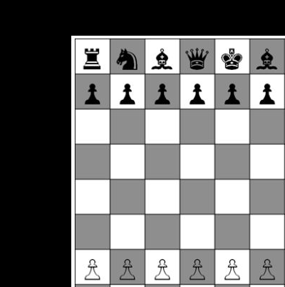
The cv2.warpAffine function takes in three arguments. The first is the image. Second is the transformation matrix for shifting. And the third is the output size.

Rotation

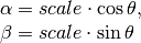
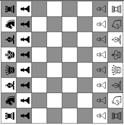
OpenCV provides rotation with an adjustable center of rotation and a scaling factor. The transformation matrix for rotation M is:

Where:


import numpy as np
import cv2
img = cv2.imread('image.jpg',0)
rows,cols = img.shape

M = cv2.getRotationMatrix2D((cols/2,rows/2),90,1)
dst = cv2.warpAffine(img,M,(cols,rows))
cv2.imshow('image',dst)
cv2.waitKey(0) & 0xFF
cv2.destroyAllWindows()

To apply this transformation matrix we used the OpenCV function cv2.getRotationMatrix2D. We scale the image by half and rotate it by 90 degrees anticlockwise.
The result is:

Affine Transformation

In this transformation all the parallel lines are kept parallel in the final image.


import numpy as np
import cv2
from matplotlib import pyplot as plt
img = cv2.imread('image.jpg')
rows,cols,ch = img.shape

pts1 = np.float32([[50,50],[200,50],[50,200]])
pts2 = np.float32([[10,100],[200,50],[100,250]])

M = cv2.getAffineTransform(pts1,pts2)

dst = cv2.warpAffine(img,M,(cols,rows))

plt.subplot(121),plt.imshow(img),plt.title('Input')
plt.subplot(122),plt.imshow(dst),plt.title('Output')
plt.show()
cv2.imshow('image',dst)
cv2.waitKey(0) & 0xFF
cv2.destroyAllWindows()

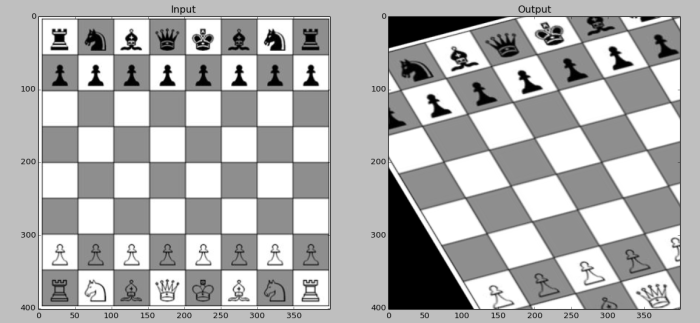
To obtain the transformation matrix we need three points from the source image and three points of the destination image to define the planes of transformation. Then using the function cv2.getAffineTransform we get a 2×3 matrix which we pass into the cv2.warpAffine function.

The result looks like this:

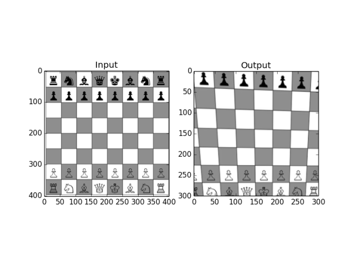
Perspective Transform

This transformation leads to change in the point of view of the image. The straight lines remain as it is. For this transformation we need 4 points from the source and output image of which 3 should be non-collinear to define a plane. From these points we define a 3×3 matrix using cv2.getPerspectiveTransform and pass the resulting matrix into cv2.warpPerspective.


import numpy as np
import cv2
from matplotlib import pyplot as plt
img = cv2.imread('image.jpg')
rows,cols,ch = img.shape

pts1 = np.float32([[56,65],[368,52],[28,387],[389,390]])
pts2 = np.float32([[0,0],[300,0],[0,300],[300,300]])

M = cv2.getPerspectiveTransform(pts1,pts2)

dst = cv2.warpPerspective(img,M,(300,300))

plt.subplot(121),plt.imshow(img),plt.title('Input')
plt.subplot(122),plt.imshow(dst),plt.title('Output')
plt.show()
plt.show()
cv2.imshow('image',dst)
cv2.waitKey(0) & 0xFF
cv2.imwrite('result.png',dst)
cv2.destroyAllWindows()


The result looks like this :

Thats all !!

OpenCV+Python:Part 3–Tracking Object using ColorSpaces

In this post I will explain how to extract a ROI using the OpenCV functions cv2.cvtColor()
The following code snippet tracks any object of blue color in the video.

import cv2
import numpy as np

cap = cv2.VideoCapture(0)

while(1):

# Take each frame
_, frame = cap.read()

# Convert BGR to HSV
hsv = cv2.cvtColor(frame, cv2.COLOR_BGR2HSV)

# define range of blue color in HSV
lower_blue = np.array([110,50,50])
upper_blue = np.array([130,255,255])

# Threshold the HSV image to get only blue colors
mask = cv2.inRange(hsv, lower_blue, upper_blue)

# Bitwise-AND mask and original image
res = cv2.bitwise_and(frame,frame, mask= mask)

cv2.imshow('frame',frame)
cv2.imshow('mask',mask)
cv2.imshow('res',res)
k = cv2.waitKey(5) & 0xFF
if k == 27:
break

cv2.destroyAllWindows()

First of all we start a normal video capture object. The using cv2.cvtColor() we change the color space from BGR to HSV. There are about 150 or more color spaces but the following code uses HSV. To know more about color spaces got to–LINK.
To know more about HSV colorspace goto–LINK.
Then we set the threshold range for the color green using the lower and upper green variables.
Then we mask every other color so that only the color green is visible.

How to find the HSV values to Track

This is a very frequent question.

>>> green = np.uint8([[[0,255,0 ]]])
>>> hsv_green = cv2.cvtColor(green,cv2.COLOR_BGR2HSV)
>>> print hsv_green


Now for the given output just take [H-10, 100,100] and [H+10, 255, 255] as lower bound and upper bound. If the result is not clear increase the range.

The output to the above code looks somthing like this.

OpenCV+Python:Part 2–Image Arithmetics

IMAGE ADDITION

You can add two images either using OpenCV: cv2.add() or Numpy: result = img1 + img2
(Both images should be of same depth and type.)There is a major difference between these two.

>>> x = np.uint8([250])
>>> y = np.uint8([10])

>>> print cv2.add(x,y) # 250+10 = 260 => 255
[[255]]

>>> print x+y # 250+10 = 260 % 256 = 4
[4]


*OpenCV provides better results

IMAGE BLENDING

Adding images using the previous method is very blunt. Using blending you can get cool transition between two images.
Blending is done by using the OpenCV function cv2.addWeighted() using the formula:
f(x)=a*img1 + (1-a)img2 + z
where a is the weight.
What we basically do is provide weights to the two images such that they mix with different intensities.

The following code adds two images with weights 0.7 and 0.3.
(Both images should be of same depth and type)

img1 = cv2.imread('img1.png')
img2 = cv2.imread('img2.jpg')

result = cv2.addWeighted(img1,0.7,img2,0.3,0) # z is taken as 0

cv2.imshow('final',result)
cv2.waitKey(0)
cv2.destroyAllWindows()


The final result looks somewhat like this:

OpenCV+Python:Part 2–Working with Images

–Access and Edit Pixel Values

All of the following steps can be performed using the Python terminal.
First of all load the image:

>>>import cv2
>>>import numpy as np
>>>img = cv2.imread('image.jpg')


To get a pixel value of a particular position:

>>>pix = img[x,y] #x,y are the coordinates
>>>print pix


To modify the pixel value of a particular point (x,y)

>>>img[x,y]=[B,G,R] #where B,G,R are integer values


A much faster method is using Numpy functions array.item() and array.itemset() to access and edit pixel values.However it only returns a scalar value.So to access the B,G,R values you need call the function array.item() separately for all.

–Image Properties
1.)>>>print image.shape
Its returns the a tuple with number of rows,columns and channels.
2.)>>>print image.size
Returns the numbers of pixels accessed by the image.
3.)>>>print img.dtype
Returns the Image datatype.

–ROI
To select a particular region of image:
>>>part = img[x1:y1,x2:y2]

To paste the selected ROI at some other location:
>>>img[p1:q1,p2:q2] = part

–Splitting and Merging Channels

If you want to split B,G,R channels or merge them back use:

>>>b,g,r = cv2.split(img)
>>>img = cv2.merge(b,g,r)


However if you want to edit a particular channel a faster method would be to use numpy.
E.g. to set all red pixels to zero:

>>> img[:,:,2] = 0


Thats all in this post..